At Palaimon, developing autoStreams involves processing massive amounts of time series data. Whether we are identifying rare events in sensor data or aligning high-frequency financial streams, the speed of our data exploration directly impacts how quickly we can iterate and deploy solutions.
The Challenge: Mining for Rare Events
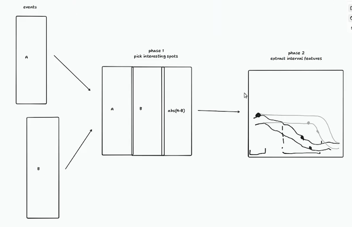
One typical workflow involves processing two event streams (e.g., different symbols or exchanges) to perform alignment and calculate statistics. We then enter a “windowing” phase, where we look back at fixed intervals (5 seconds to 5 minutes) around interesting points to extract features.
The scale of this data is significant:
- Individual assets: Up to 20 million events per year.
- Total volume: 50-100 GB for a typical use case (hundreds of assets).
- Goal: Mine billions of events to find the “needle in the haystack.”
Why Naive Pandas Isn’t Enough
For our initial exploration, we used a “naive” Pandas approach. While Pandas is the industry standard, its single-threaded nature becomes a bottleneck as data scales.
In our benchmarks (processing 4 assets over 1 year), the naive implementation took about 10 minutes. Scaling this to 100 assets would take over 16 hours (1000 minutes), making interactive exploration impossible.
Exploring the Optimization Landscape
We investigated several paths to speed up our pipeline:
1. Naive Pandas
The baseline. Easy to write, but slow for large-scale windowing and grouping operations.
0/2 process: 100%|█| 4/4 [03:53<00:00, 58.29s/it]
1/2 process: 100%|█| 4/4 [05:23<00:00, 80.87s/it]
2. GPU Acceleration (cuDF / Cooder / FireDax)
We tried running our naive Pandas code on GPU-accelerated frameworks like cuDF (via cudf.pandas) and others. Surprisingly, performance degraded. The overhead of data transfer to the GPU and the presence of non-vectorizable operations meant the GPU was actually slower than the CPU.
0/2 process: 100%|█| 4/4 [05:33<00:00, 83.30s/it]
1/2 process: 100%|█| 4/4 [07:41<00:00, 115.44s/it]
3. Optimized Pandas
By refactoring the Pandas code to address simple bottlenecks (e.g., pre-calculating weighted prices and reducing the complexity of groupby.apply), we achieved a significant speedup.
0/2 process: 100%|█| 4/4 [01:13<00:00, 18.43s/it]
1/2 process: 100%|█| 4/4 [01:21<00:00, 20.36s/it]
4. Polars (CPU)
Switching to Polars was a game-changer. Polars’ expression engine and built-in multithreading allowed us to process the same data in seconds.
0/2 process: 100%|█| 4/4 [00:08<00:00,  2.07s/it]
1/2 process: 100%|█| 4/4 [00:10<00:00,  2.66s/it]
5. Polars (GPU)
We also experimented with the new Polars GPU engine. While it showed similar performance to the CPU version for this specific task, it opens the door for even larger datasets where memory bandwidth becomes the primary bottleneck.
0/2 process: 100%|█| 4/4 [00:09<00:00,  2.38s/it]
1/2 process: 100%|█| 4/4 [00:11<00:00,  2.78s/it]
Benchmark Results
| Framework | Execution Time (4 assets, 1 year) | Speedup |
|---|---|---|
| Naive Pandas | ~556s | 1x |
| Optimized Pandas | ~154s | ~3.6x |
| Polars (CPU) | ~18s | ~30x |
| Polars (GPU) | ~20s | ~28x |
Note: Timings are the sum of two processing batches (1/2 year each).
Conclusion
For interactive data exploration at the 50-100 GB scale, Polars is currently our tool of choice. It provides the performance of a distributed system on a single machine without the complexity of GPU drivers or specialized hardware. While GPU acceleration shows promise, the efficiency of the Polars CPU engine is often more than enough to turn a “coffee break” task into an “instant” one.